计算机视觉中的迁移学习教程
在本教程中,您将学习如何使用迁移学习训练卷积神经网络进行图像分类。您可以在 cs231n 笔记 中阅读更多关于迁移学习的内容。
引用这些笔记:
在实际应用中,很少有人从头开始训练整个卷积神经网络(使用随机初始化),因为拥有足够大规模数据集的情况相对较少。相反,常见的做法是在一个非常大的数据集(例如ImageNet,包含120万张图像和1000个类别)上预训练一个卷积神经网络,然后将该网络作为初始化模型或固定特征提取器,应用于目标任务。
这两种主要的迁移学习场景如下所示:
-
微调卷积神经网络: 我们不是随机初始化网络,而是使用预训练的网络(例如在 ImageNet 1000 数据集上训练的网络)进行初始化。其余的训练过程与常规相同。
-
将卷积神经网络作为固定特征提取器: 在这里,我们将冻结网络中除最后一个全连接层之外的所有权重。最后的全连接层被替换为一个随机权重的新层,并仅训练这一层。
# License: BSD
# Author: Sasank Chilamkurthy

importtorch
importtorch.nnasnn
importtorch.optimasoptim
fromtorch.optimimport lr_scheduler
importtorch.backends.cudnnascudnn
importnumpyasnp
importtorchvision
fromtorchvisionimport datasets, models, transforms
importmatplotlib.pyplotasplt
importtime
importos
fromPILimport Image
fromtempfileimport TemporaryDirectory

cudnn.benchmark = True
plt.ion()   # interactive mode
<contextlib.ExitStack object at 0x7fc173de6b60>
加载数据
我们将使用 torchvision 和 torch.utils.data 包来加载数据。
我们今天要解决的问题是训练一个模型来分类蚂蚁和蜜蜂。我们各有大约 120 张蚂蚁和蜜蜂的训练图像。每个类别还有 75 张验证图像。通常来说,如果从头开始训练,这是一个非常小的数据集,难以进行泛化。但由于我们使用了迁移学习,应该能够较好地实现泛化。
这个数据集是 ImageNet 的一个非常小的子集。
从这里下载数据并将其解压到当前目录。
# Data augmentation and normalization for training
# Just normalization for validation
data_transforms = {
    'train': transforms.Compose([
        transforms.RandomResizedCrop(224),
        transforms.RandomHorizontalFlip(),
        transforms.ToTensor(),
        transforms.Normalize([0.485, 0.456, 0.406], [0.229, 0.224, 0.225])
    ]),
    'val': transforms.Compose([
        transforms.Resize(256),
        transforms.CenterCrop(224),
        transforms.ToTensor(),
        transforms.Normalize([0.485, 0.456, 0.406], [0.229, 0.224, 0.225])
    ]),
}

data_dir = 'data/hymenoptera_data'
image_datasets = {x: datasets.ImageFolder(os.path.join(data_dir, x),
                                          data_transforms[x])
                  for x in ['train', 'val']}
dataloaders = {x: torch.utils.data.DataLoader(image_datasets[x], batch_size=4,
                                             shuffle=True, num_workers=4)
              for x in ['train', 'val']}
dataset_sizes = {x: len(image_datasets[x]) for x in ['train', 'val']}
class_names = image_datasets['train'].classes

# We want to be able to train our model on an `accelerator <https://pytorch.org/docs/stable/torch.html#accelerators>`__
# such as CUDA, MPS, MTIA, or XPU. If the current accelerator is available, we will use it. Otherwise, we use the CPU.

device = torch.accelerator.current_accelerator().type if torch.accelerator.is_available() else "cpu"
print(f"Using {device} device")
Using cuda device
可视化一些图像
让我们可视化一些训练图像,以便更好地理解数据增强的效果。
defimshow(inp, title=None):
"""Display image for Tensor."""
    inp = inp.numpy().transpose((1, 2, 0))
    mean = np.array([0.485, 0.456, 0.406])
    std = np.array([0.229, 0.224, 0.225])
    inp = std * inp + mean
    inp = np.clip(inp, 0, 1)
    plt.imshow(inp)
    if title is not None:
        plt.title(title)
    plt.pause(0.001)  # pause a bit so that plots are updated


# Get a batch of training data
inputs, classes = next(iter(dataloaders['train']))

# Make a grid from batch
out = torchvision.utils.make_grid(inputs)

imshow(out, title=[class_names[x] for x in classes])
训练模型
现在,让我们编写一个通用函数来训练模型。这里,我们将演示:
-
调度学习率
-
保存最佳模型
在以下内容中,参数 scheduler 是来自 torch.optim.lr_scheduler 的学习率调度器对象。
deftrain_model(model, criterion, optimizer, scheduler, num_epochs=25):
    since = time.time()

    # Create a temporary directory to save training checkpoints
    with TemporaryDirectory() as tempdir:
        best_model_params_path = os.path.join(tempdir, 'best_model_params.pt')

        torch.save(model.state_dict(), best_model_params_path)
        best_acc = 0.0

        for epoch in range(num_epochs):
            print(f'Epoch {epoch}/{num_epochs-1}')
            print('-' * 10)

            # Each epoch has a training and validation phase
            for phase in ['train', 'val']:
                if phase == 'train':
                    model.train()  # Set model to training mode
                else:
                    model.eval()   # Set model to evaluate mode

                running_loss = 0.0
                running_corrects = 0

                # Iterate over data.
                for inputs, labels in dataloaders[phase]:
                    inputs = inputs.to(device)
                    labels = labels.to(device)

                    # zero the parameter gradients
                    optimizer.zero_grad()

                    # forward
                    # track history if only in train
                    with torch.set_grad_enabled(phase == 'train'):
                        outputs = model(inputs)
                        _, preds = torch.max(outputs, 1)
                        loss = criterion(outputs, labels)

                        # backward + optimize only if in training phase
                        if phase == 'train':
                            loss.backward()
                            optimizer.step()

                    # statistics
                    running_loss += loss.item() * inputs.size(0)
                    running_corrects += torch.sum(preds == labels.data)
                if phase == 'train':
                    scheduler.step()

                epoch_loss = running_loss / dataset_sizes[phase]
                epoch_acc = running_corrects.double() / dataset_sizes[phase]

                print(f'{phase} Loss: {epoch_loss:.4f} Acc: {epoch_acc:.4f}')

                # deep copy the model
                if phase == 'val' and epoch_acc > best_acc:
                    best_acc = epoch_acc
                    torch.save(model.state_dict(), best_model_params_path)

            print()

        time_elapsed = time.time() - since
        print(f'Training complete in {time_elapsed//60:.0f}m {time_elapsed%60:.0f}s')
        print(f'Best val Acc: {best_acc:4f}')

        # load best model weights
        model.load_state_dict(torch.load(best_model_params_path, weights_only=True))
    return model
可视化模型预测结果
用于显示几张图像预测的通用函数
defvisualize_model(model, num_images=6):
    was_training = model.training
    model.eval()
    images_so_far = 0
    fig = plt.figure()

    with torch.no_grad():
        for i, (inputs, labels) in enumerate(dataloaders['val']):
            inputs = inputs.to(device)
            labels = labels.to(device)

            outputs = model(inputs)
            _, preds = torch.max(outputs, 1)

            for j in range(inputs.size()[0]):
                images_so_far += 1
                ax = plt.subplot(num_images//2, 2, images_so_far)
                ax.axis('off')
                ax.set_title(f'predicted: {class_names[preds[j]]}')
                imshow(inputs.cpu().data[j])

                if images_so_far == num_images:
                    model.train(mode=was_training)
                    return
        model.train(mode=was_training)
微调卷积神经网络
加载预训练模型并重置最后的全连接层。
model_ft = models.resnet18(weights='IMAGENET1K_V1')
num_ftrs = model_ft.fc.in_features
# Here the size of each output sample is set to 2.
# Alternatively, it can be generalized to ``nn.Linear(num_ftrs, len(class_names))``.
model_ft.fc = nn.Linear(num_ftrs, 2)

model_ft = model_ft.to(device)

criterion = nn.CrossEntropyLoss()

# Observe that all parameters are being optimized
optimizer_ft = optim.SGD(model_ft.parameters(), lr=0.001, momentum=0.9)

# Decay LR by a factor of 0.1 every 7 epochs
exp_lr_scheduler = lr_scheduler.StepLR(optimizer_ft, step_size=7, gamma=0.1)
Downloading: "https://download.pytorch.org/models/resnet18-f37072fd.pth" to /var/lib/ci-user/.cache/torch/hub/checkpoints/resnet18-f37072fd.pth

  0%|          | 0.00/44.7M [00:00<?, ?B/s]
 47%|####6     | 20.9M/44.7M [00:00<00:00, 218MB/s]
 93%|#########3| 41.8M/44.7M [00:00<00:00, 218MB/s]
100%|##########| 44.7M/44.7M [00:00<00:00, 218MB/s]
训练和评估
在 CPU 上大约需要 15-25 分钟。而在 GPU 上,则不到一分钟即可完成。
model_ft = train_model(model_ft, criterion, optimizer_ft, exp_lr_scheduler,
                       num_epochs=25)
Epoch 0/24
*---------
train Loss: 0.4770 Acc: 0.7541
val Loss: 0.2993 Acc: 0.8889

Epoch 1/24
*---------
train Loss: 0.5462 Acc: 0.7746
val Loss: 0.6804 Acc: 0.7255

Epoch 2/24
*---------
train Loss: 0.4351 Acc: 0.8197
val Loss: 0.2319 Acc: 0.8889

Epoch 3/24
*---------
train Loss: 0.5622 Acc: 0.8033
val Loss: 0.3092 Acc: 0.8889

Epoch 4/24
*---------
train Loss: 0.3790 Acc: 0.8607
val Loss: 0.2291 Acc: 0.9150

Epoch 5/24
*---------
train Loss: 0.4498 Acc: 0.8238
val Loss: 0.2667 Acc: 0.8889

Epoch 6/24
*---------
train Loss: 0.3996 Acc: 0.8320
val Loss: 0.2539 Acc: 0.9150

Epoch 7/24
*---------
train Loss: 0.3644 Acc: 0.8607
val Loss: 0.2067 Acc: 0.9020

Epoch 8/24
*---------
train Loss: 0.2031 Acc: 0.9303
val Loss: 0.2134 Acc: 0.8954

Epoch 9/24
*---------
train Loss: 0.2553 Acc: 0.8730
val Loss: 0.2153 Acc: 0.9150

Epoch 10/24
*---------
train Loss: 0.3431 Acc: 0.8689
val Loss: 0.1867 Acc: 0.9150

Epoch 11/24
*---------
train Loss: 0.3152 Acc: 0.8484
val Loss: 0.2464 Acc: 0.9020

Epoch 12/24
*---------
train Loss: 0.2363 Acc: 0.8893
val Loss: 0.1982 Acc: 0.9216

Epoch 13/24
*---------
train Loss: 0.2775 Acc: 0.8689
val Loss: 0.1871 Acc: 0.9216

Epoch 14/24
*---------
train Loss: 0.2671 Acc: 0.8770
val Loss: 0.2233 Acc: 0.9020

Epoch 15/24
*---------
train Loss: 0.3027 Acc: 0.8730
val Loss: 0.2656 Acc: 0.8758

Epoch 16/24
*---------
train Loss: 0.2073 Acc: 0.9139
val Loss: 0.2040 Acc: 0.9150

Epoch 17/24
*---------
train Loss: 0.2469 Acc: 0.8893
val Loss: 0.1884 Acc: 0.9150

Epoch 18/24
*---------
train Loss: 0.2636 Acc: 0.8811
val Loss: 0.2194 Acc: 0.9020

Epoch 19/24
*---------
train Loss: 0.2010 Acc: 0.9262
val Loss: 0.1930 Acc: 0.9150

Epoch 20/24
*---------
train Loss: 0.2605 Acc: 0.9098
val Loss: 0.1849 Acc: 0.9216

Epoch 21/24
*---------
train Loss: 0.2451 Acc: 0.8893
val Loss: 0.2322 Acc: 0.8954

Epoch 22/24
*---------
train Loss: 0.2937 Acc: 0.8730
val Loss: 0.1930 Acc: 0.9281

Epoch 23/24
*---------
train Loss: 0.2685 Acc: 0.8689
val Loss: 0.2080 Acc: 0.9150

Epoch 24/24
*---------
train Loss: 0.2743 Acc: 0.8852
val Loss: 0.1978 Acc: 0.9281

Training complete in 1m 4s
Best val Acc: 0.928105
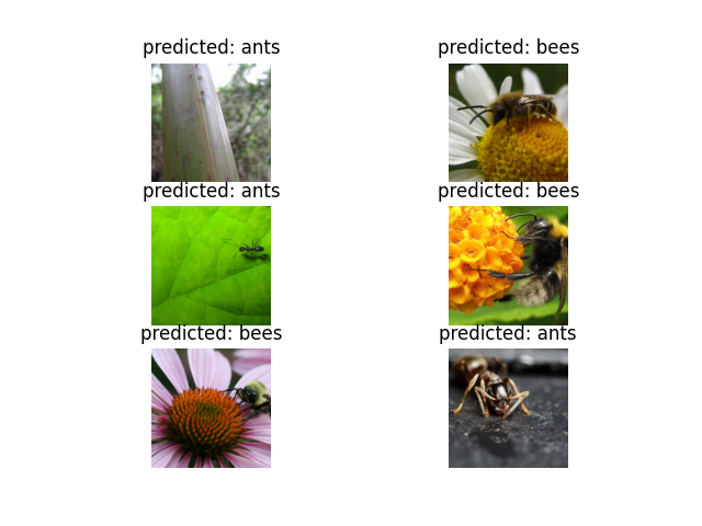
visualize_model(model_ft)
将卷积神经网络作为固定特征提取器
在这里,我们需要冻结除最后一层之外的所有网络。我们需要将 requires_grad 设置为 False 来冻结参数,以便在 backward() 中不计算梯度。
您可以在文档 这里 中阅读更多相关内容。
model_conv = torchvision.models.resnet18(weights='IMAGENET1K_V1')
for param in model_conv.parameters():
    param.requires_grad = False

# Parameters of newly constructed modules have requires_grad=True by default
num_ftrs = model_conv.fc.in_features
model_conv.fc = nn.Linear(num_ftrs, 2)

model_conv = model_conv.to(device)

criterion = nn.CrossEntropyLoss()

# Observe that only parameters of final layer are being optimized as
# opposed to before.
optimizer_conv = optim.SGD(model_conv.fc.parameters(), lr=0.001, momentum=0.9)

# Decay LR by a factor of 0.1 every 7 epochs
exp_lr_scheduler = lr_scheduler.StepLR(optimizer_conv, step_size=7, gamma=0.1)
训练与评估
在 CPU 上,这将比之前的情况节省大约一半的时间。这是预期的,因为大部分网络不需要计算梯度。然而,前向传播仍然需要计算。
model_conv = train_model(model_conv, criterion, optimizer_conv,
                         exp_lr_scheduler, num_epochs=25)
Epoch 0/24
*---------
train Loss: 0.6996 Acc: 0.6516
val Loss: 0.2014 Acc: 0.9346

Epoch 1/24
*---------
train Loss: 0.4233 Acc: 0.8033
val Loss: 0.2656 Acc: 0.8758

Epoch 2/24
*---------
train Loss: 0.4603 Acc: 0.7869
val Loss: 0.1847 Acc: 0.9477

Epoch 3/24
*---------
train Loss: 0.3096 Acc: 0.8566
val Loss: 0.1747 Acc: 0.9477

Epoch 4/24
*---------
train Loss: 0.4427 Acc: 0.8156
val Loss: 0.1630 Acc: 0.9477

Epoch 5/24
*---------
train Loss: 0.5505 Acc: 0.7828
val Loss: 0.1643 Acc: 0.9477

Epoch 6/24
*---------
train Loss: 0.3004 Acc: 0.8607
val Loss: 0.1744 Acc: 0.9542

Epoch 7/24
*---------
train Loss: 0.4083 Acc: 0.8361
val Loss: 0.1892 Acc: 0.9412

Epoch 8/24
*---------
train Loss: 0.4483 Acc: 0.7910
val Loss: 0.1984 Acc: 0.9477

Epoch 9/24
*---------
train Loss: 0.3335 Acc: 0.8279
val Loss: 0.1942 Acc: 0.9412

Epoch 10/24
*---------
train Loss: 0.2413 Acc: 0.8934
val Loss: 0.2001 Acc: 0.9477

Epoch 11/24
*---------
train Loss: 0.3107 Acc: 0.8689
val Loss: 0.1801 Acc: 0.9412

Epoch 12/24
*---------
train Loss: 0.3032 Acc: 0.8689
val Loss: 0.1669 Acc: 0.9477

Epoch 13/24
*---------
train Loss: 0.3587 Acc: 0.8525
val Loss: 0.1900 Acc: 0.9477

Epoch 14/24
*---------
train Loss: 0.2771 Acc: 0.8893
val Loss: 0.2317 Acc: 0.9216

Epoch 15/24
*---------
train Loss: 0.3064 Acc: 0.8852
val Loss: 0.1909 Acc: 0.9477

Epoch 16/24
*---------
train Loss: 0.4243 Acc: 0.8238
val Loss: 0.2227 Acc: 0.9346

Epoch 17/24
*---------
train Loss: 0.3297 Acc: 0.8238
val Loss: 0.1916 Acc: 0.9412

Epoch 18/24
*---------
train Loss: 0.4235 Acc: 0.8238
val Loss: 0.1766 Acc: 0.9477

Epoch 19/24
*---------
train Loss: 0.2500 Acc: 0.8934
val Loss: 0.2003 Acc: 0.9477

Epoch 20/24
*---------
train Loss: 0.2413 Acc: 0.8934
val Loss: 0.1821 Acc: 0.9477

Epoch 21/24
*---------
train Loss: 0.3762 Acc: 0.8115
val Loss: 0.1842 Acc: 0.9412

Epoch 22/24
*---------
train Loss: 0.3485 Acc: 0.8566
val Loss: 0.2166 Acc: 0.9281

Epoch 23/24
*---------
train Loss: 0.3625 Acc: 0.8361
val Loss: 0.1747 Acc: 0.9412

Epoch 24/24
*---------
train Loss: 0.3840 Acc: 0.8320
val Loss: 0.1768 Acc: 0.9412

Training complete in 0m 32s
Best val Acc: 0.954248
visualize_model(model_conv)

plt.ioff()
plt.show()

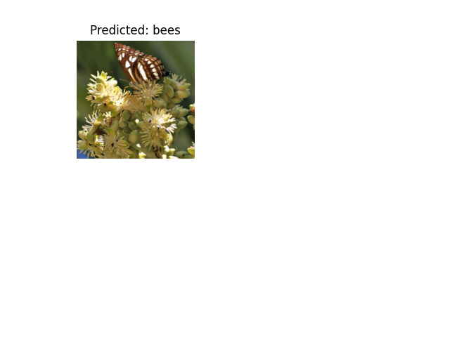
自定义图像推理
使用训练好的模型对自定义图像进行预测,并将预测的类别标签与图像一起可视化。
defvisualize_model_predictions(model,img_path):
    was_training = model.training
    model.eval()

    img = Image.open(img_path)
    img = data_transforms['val'](img)
    img = img.unsqueeze(0)
    img = img.to(device)

    with torch.no_grad():
        outputs = model(img)
        _, preds = torch.max(outputs, 1)

        ax = plt.subplot(2,2,1)
        ax.axis('off')
        ax.set_title(f'Predicted: {class_names[preds[0]]}')
        imshow(img.cpu().data[0])

        model.train(mode=was_training)
visualize_model_predictions(
    model_conv,
    img_path='data/hymenoptera_data/val/bees/72100438_73de9f17af.jpg'
)

plt.ioff()
plt.show()
深入学习
如果您想了解更多关于迁移学习的应用,请查看我们的计算机视觉量化迁移学习教程。