知识蒸馏教程

知识蒸馏是一种技术，它能够将知识从大型、计算成本高的模型转移到较小的模型，而不会损失有效性。这使得在性能较低的硬件上部署成为可能，从而加快评估速度并提高效率。

在本教程中，我们将运行一系列实验，旨在通过使用一个更强大的网络作为教师模型，来提高一个轻量级神经网络的准确性。轻量级网络的计算成本和速度将保持不变，我们的干预仅关注其权重，而不影响其前向传播。该技术可以应用于无人机或手机等设备。在本教程中，我们不使用任何外部包，因为所需的一切都可以在 torch 和 torchvision 中找到。

在本教程中，您将学习：

如何修改模型类以提取隐藏表示并将其用于进一步计算
如何修改 PyTorch 中的常规训练循环，以在分类的交叉熵损失之上加入额外的损失
如何通过使用更复杂的模型作为教师来提高轻量级模型的性能

先决条件

1 个 GPU，4GB 内存
PyTorch v2.0 或更高版本
CIFAR-10 数据集（由脚本下载并保存在名为 /data 的目录中）

importtorch
importtorch.nnasnn
importtorch.optimasoptim
importtorchvision.transformsastransforms
importtorchvision.datasetsasdatasets

# Check if the current `accelerator <https://pytorch.org/docs/stable/torch.html#accelerators>`__
# is available, and if not, use the CPU
device = torch.accelerator.current_accelerator().type if torch.accelerator.is_available() else "cpu"
print(f"Using {device} device")

Using cuda device

加载 CIFAR-10 数据集

CIFAR-10 是一个包含十个类别的常用图像数据集。我们的目标是为每张输入图像预测出以下类别之一。

../_static/img/cifar10.png

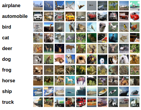
CIFAR-10 图像示例

输入图像是RGB格式的，因此它们有3个通道，并且每张图像的尺寸为32x32像素。基本上，每张图像由3 x 32 x 32 = 3072个数值描述，这些数值的范围在0到255之间。在神经网络中，常见的做法是对输入进行归一化，这样做有多种原因，包括避免常用激活函数的饱和以及提高数值稳定性。我们的归一化过程包括减去均值并除以每个通道的标准差。张量“mean=[0.485, 0.456, 0.406]”和“std=[0.229, 0.224, 0.225]”已经预先计算好了，它们代表了CIFAR-10数据集中预定义训练集子集中每个通道的均值和标准差。需要注意的是，我们在测试集上也使用了这些值，而没有从头重新计算均值和标准差。这是因为网络是基于上述数值进行减法和除法处理后得到的特征进行训练的，我们希望保持一致性。此外，在实际情况中，我们无法计算测试集的均值和标准差，因为根据我们的假设，这些数据在此时是不可访问的。

最后，我们通常将这个保留的数据集称为验证集，并在优化模型在验证集上的性能之后，使用另一个称为测试集的独立数据集。这样做是为了避免基于单一指标的贪婪和有偏优化来选择模型。

# Below we are preprocessing data for CIFAR-10. We use an arbitrary batch size of 128.
transforms_cifar = transforms.Compose([
    transforms.ToTensor(),
    transforms.Normalize(mean=[0.485, 0.456, 0.406], std=[0.229, 0.224, 0.225]),
])

# Loading the CIFAR-10 dataset:
train_dataset = datasets.CIFAR10(root='./data', train=True, download=True, transform=transforms_cifar)
test_dataset = datasets.CIFAR10(root='./data', train=False, download=True, transform=transforms_cifar)

本节仅适用于希望快速获得结果的CPU用户。如果您只对小型实验感兴趣，请使用此选项。请记住，使用任何GPU时，代码的运行速度都会相当快。从训练/测试数据集中仅选择前num_images_to_keep张图像
#from torch.utils.data import Subset
#num_images_to_keep = 2000
#train_dataset = Subset(train_dataset, range(min(num_images_to_keep, 50_000)))
#test_dataset = Subset(test_dataset, range(min(num_images_to_keep, 10_000)))

#Dataloaders
train_loader = torch.utils.data.DataLoader(train_dataset, batch_size=128, shuffle=True, num_workers=2)
test_loader = torch.utils.data.DataLoader(test_dataset, batch_size=128, shuffle=False, num_workers=2)

定义模型类和工具函数

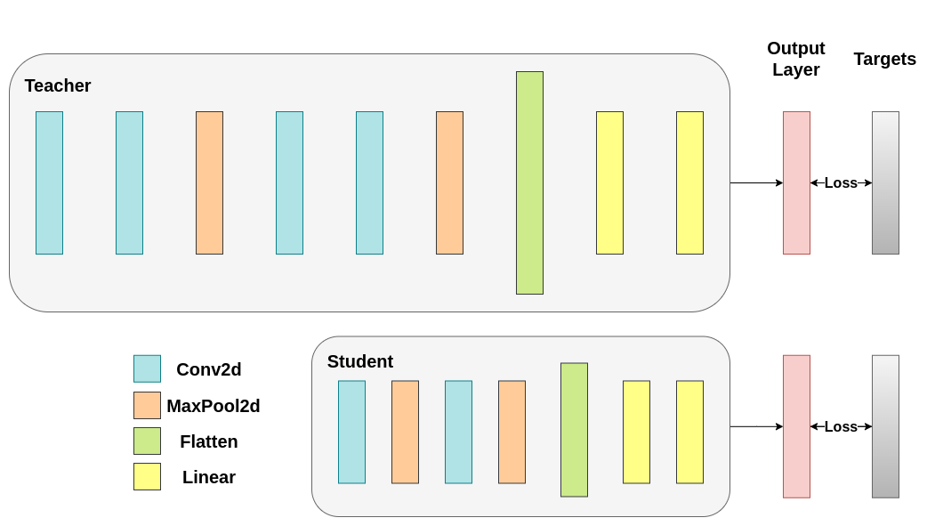
接下来，我们需要定义我们的模型类。这里需要设置几个用户定义的参数。我们使用了两种不同的架构，在实验中保持滤波器的数量不变，以确保公平比较。这两种架构都是卷积神经网络（CNNs），卷积层的数量不同，作为特征提取器，后面跟着一个具有10个类别的分类器。学生的滤波器数量和神经元数量较少。

# Deeper neural network class to be used as teacher:
classDeepNN(nn.Module):
    def__init__(self, num_classes=10):
        super(DeepNN, self).__init__()
        self.features = nn.Sequential(
            nn.Conv2d(3, 128, kernel_size=3, padding=1),
            nn.ReLU(),
            nn.Conv2d(128, 64, kernel_size=3, padding=1),
            nn.ReLU(),
            nn.MaxPool2d(kernel_size=2, stride=2),
            nn.Conv2d(64, 64, kernel_size=3, padding=1),
            nn.ReLU(),
            nn.Conv2d(64, 32, kernel_size=3, padding=1),
            nn.ReLU(),
            nn.MaxPool2d(kernel_size=2, stride=2),
        )
        self.classifier = nn.Sequential(
            nn.Linear(2048, 512),
            nn.ReLU(),
            nn.Dropout(0.1),
            nn.Linear(512, num_classes)
        )

    defforward(self, x):
        x = self.features(x)
        x = torch.flatten(x, 1)
        x = self.classifier(x)
        return x

# Lightweight neural network class to be used as student:
classLightNN(nn.Module):
    def__init__(self, num_classes=10):
        super(LightNN, self).__init__()
        self.features = nn.Sequential(
            nn.Conv2d(3, 16, kernel_size=3, padding=1),
            nn.ReLU(),
            nn.MaxPool2d(kernel_size=2, stride=2),
            nn.Conv2d(16, 16, kernel_size=3, padding=1),
            nn.ReLU(),
            nn.MaxPool2d(kernel_size=2, stride=2),
        )
        self.classifier = nn.Sequential(
            nn.Linear(1024, 256),
            nn.ReLU(),
            nn.Dropout(0.1),
            nn.Linear(256, num_classes)
        )

    defforward(self, x):
        x = self.features(x)
        x = torch.flatten(x, 1)
        x = self.classifier(x)
        return x

我们使用两个函数来帮助我们生成并评估原始分类任务的结果。其中一个函数名为 train，它接受以下参数：

model: 一个模型实例，通过此函数进行训练（更新其权重）。
train_loader: 我们在上面定义了 train_loader，它的任务是将数据输入到模型中。
epochs: 我们循环遍历数据集的次数。
learning_rate: 学习率决定了我们向收敛方向迈出的步长大小。步长过大或过小都可能带来不利影响。
device: 确定运行工作负载的设备。根据可用性，可以是 CPU 或 GPU。

我们的测试函数类似，但它将使用 test_loader 来加载测试集中的图像。

../_static/img/knowledge_distillation/ce_only.png

使用交叉熵训练两个网络。学生网络将作为基线：

deftrain(model, train_loader, epochs, learning_rate, device):
    criterion = nn.CrossEntropyLoss()
    optimizer = optim.Adam(model.parameters(), lr=learning_rate)

    model.train()

    for epoch in range(epochs):
        running_loss = 0.0
        for inputs, labels in train_loader:
            # inputs: A collection of batch_size images
            # labels: A vector of dimensionality batch_size with integers denoting class of each image
            inputs, labels = inputs.to(device), labels.to(device)

            optimizer.zero_grad()
            outputs = model(inputs)

            # outputs: Output of the network for the collection of images. A tensor of dimensionality batch_size x num_classes
            # labels: The actual labels of the images. Vector of dimensionality batch_size
            loss = criterion(outputs, labels)
            loss.backward()
            optimizer.step()

            running_loss += loss.item()

        print(f"Epoch {epoch+1}/{epochs}, Loss: {running_loss/len(train_loader)}")

deftest(model, test_loader, device):
    model.to(device)
    model.eval()

    correct = 0
    total = 0

    with torch.no_grad():
        for inputs, labels in test_loader:
            inputs, labels = inputs.to(device), labels.to(device)

            outputs = model(inputs)
            _, predicted = torch.max(outputs.data, 1)

            total += labels.size(0)
            correct += (predicted == labels).sum().item()

    accuracy = 100 * correct / total
    print(f"Test Accuracy: {accuracy:.2f}%")
    return accuracy

交叉熵训练

为了确保可重复性，我们需要设置 torch 的手动种子。我们使用不同的方法训练网络，因此为了公平比较，用相同的权重初始化网络是有意义的。首先使用交叉熵训练教师网络：

torch.manual_seed(42)
nn_deep = DeepNN(num_classes=10).to(device)
train(nn_deep, train_loader, epochs=10, learning_rate=0.001, device=device)
test_accuracy_deep = test(nn_deep, test_loader, device)

# Instantiate the lightweight network:
torch.manual_seed(42)
nn_light = LightNN(num_classes=10).to(device)

Epoch 1/10, Loss: 1.3271721180747538
Epoch 2/10, Loss: 0.8677293405203563
Epoch 3/10, Loss: 0.6773818351728532
Epoch 4/10, Loss: 0.533347406731847
Epoch 5/10, Loss: 0.41782562823399255
Epoch 6/10, Loss: 0.3038525020756075
Epoch 7/10, Loss: 0.2176617298589643
Epoch 8/10, Loss: 0.16839655402028347
Epoch 9/10, Loss: 0.13820644220351563
Epoch 10/10, Loss: 0.11872172021709593
Test Accuracy: 74.59%

我们实例化了一个更轻量级的网络模型来比较它们的性能。反向传播对权重初始化非常敏感，因此我们需要确保这两个网络具有完全相同的初始化。

torch.manual_seed(42)
new_nn_light = LightNN(num_classes=10).to(device)

为了确保我们已经创建了第一个网络的副本，我们检查其第一层的范数。如果匹配，那么我们可以安全地得出结论，这两个网络确实是相同的。

# Print the norm of the first layer of the initial lightweight model
print("Norm of 1st layer of nn_light:", torch.norm(nn_light.features[0].weight).item())
# Print the norm of the first layer of the new lightweight model
print("Norm of 1st layer of new_nn_light:", torch.norm(new_nn_light.features[0].weight).item())

Norm of 1st layer of nn_light: 2.327361822128296
Norm of 1st layer of new_nn_light: 2.327361822128296

打印每个模型中的参数总数：

total_params_deep = "{:,}".format(sum(p.numel() for p in nn_deep.parameters()))
print(f"DeepNN parameters: {total_params_deep}")
total_params_light = "{:,}".format(sum(p.numel() for p in nn_light.parameters()))
print(f"LightNN parameters: {total_params_light}")

DeepNN parameters: 1,186,986
LightNN parameters: 267,738

使用交叉熵损失训练和测试轻量级网络：

train(nn_light, train_loader, epochs=10, learning_rate=0.001, device=device)
test_accuracy_light_ce = test(nn_light, test_loader, device)

Epoch 1/10, Loss: 1.4694825563284442
Epoch 2/10, Loss: 1.1577004929027899
Epoch 3/10, Loss: 1.0258077334260087
Epoch 4/10, Loss: 0.9231916531882323
Epoch 5/10, Loss: 0.8473384543453031
Epoch 6/10, Loss: 0.777854927055671
Epoch 7/10, Loss: 0.7123624658035805
Epoch 8/10, Loss: 0.6548263956518734
Epoch 9/10, Loss: 0.5991184807494473
Epoch 10/10, Loss: 0.5516214456094806
Test Accuracy: 70.66%

正如我们所看到的，基于测试准确率，我们现在可以将用作教师的深层网络与作为学生轻量级网络进行比较。到目前为止，我们的学生尚未与教师进行交互，因此这一性能是由学生自身实现的。到目前为止的指标可以通过以下代码行查看：

print(f"Teacher accuracy: {test_accuracy_deep:.2f}%")
print(f"Student accuracy: {test_accuracy_light_ce:.2f}%")

Teacher accuracy: 74.59%
Student accuracy: 70.66%

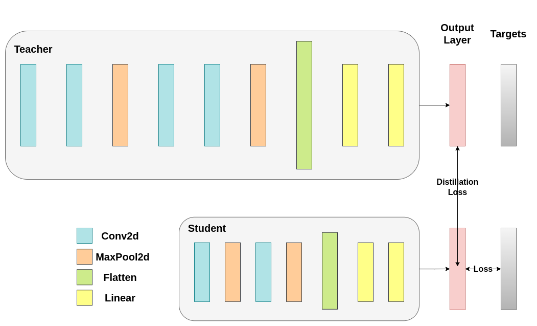
知识蒸馏运行

现在，让我们尝试通过引入教师网络来提高学生网络的测试准确率。知识蒸馏是一种实现这一目标的直接方法，它基于两个网络都会输出类别概率分布的事实。因此，两个网络具有相同数量的输出神经元。该方法通过在传统的交叉熵损失中引入一个额外的损失来实现，该损失基于教师网络的 softmax 输出。假设是，经过适当训练的教师网络的输出激活包含额外的信息，这些信息可以被学生网络在训练过程中利用。原始研究表明，利用 soft 目标中较小概率的比率可以帮助实现深度神经网络的基本目标，即在数据上创建相似性结构，使得相似的对象在映射空间中更接近。例如，在 CIFAR-10 数据集中，如果卡车带有轮子，它可能会被误认为是汽车或飞机，但不太可能被误认为是狗。因此，有理由假设有价值的信息不仅存在于经过适当训练的模型的顶部预测中，还存在于整个输出分布中。然而，仅靠交叉熵并不能充分挖掘这些信息，因为非预测类的激活往往非常小，导致传播的梯度无法有意义地改变权重以构建这种理想的向量空间。

在继续定义我们的第一个引入师生动态的辅助函数时，我们需要包含一些额外的参数：

T: 温度控制输出分布的平滑度。较大的 T 会使分布更加平滑，因此较小的概率会得到更大的提升。
soft_target_loss_weight: 分配给即将引入的额外目标的权重。
ce_loss_weight: 分配给交叉熵的权重。调整这些权重可以推动网络朝着优化某一目标的方向发展。

../_static/img/knowledge_distillation/distillation_output_loss.png

蒸馏损失是根据网络的 logits 计算的。它只向学生网络返回梯度：

deftrain_knowledge_distillation(teacher, student, train_loader, epochs, learning_rate, T, soft_target_loss_weight, ce_loss_weight, device):
    ce_loss = nn.CrossEntropyLoss()
    optimizer = optim.Adam(student.parameters(), lr=learning_rate)

    teacher.eval()  # Teacher set to evaluation mode
    student.train() # Student to train mode

    for epoch in range(epochs):
        running_loss = 0.0
        for inputs, labels in train_loader:
            inputs, labels = inputs.to(device), labels.to(device)

            optimizer.zero_grad()

            # Forward pass with the teacher model - do not save gradients here as we do not change the teacher's weights
            with torch.no_grad():
                teacher_logits = teacher(inputs)

            # Forward pass with the student model
            student_logits = student(inputs)

            #Soften the student logits by applying softmax first and log() second
            soft_targets = nn.functional.softmax(teacher_logits / T, dim=-1)
            soft_prob = nn.functional.log_softmax(student_logits / T, dim=-1)

            # Calculate the soft targets loss. Scaled by T**2 as suggested by the authors of the paper "Distilling the knowledge in a neural network"
            soft_targets_loss = torch.sum(soft_targets * (soft_targets.log() - soft_prob)) / soft_prob.size()[0] * (T**2)

            # Calculate the true label loss
            label_loss = ce_loss(student_logits, labels)

            # Weighted sum of the two losses
            loss = soft_target_loss_weight * soft_targets_loss + ce_loss_weight * label_loss

            loss.backward()
            optimizer.step()

            running_loss += loss.item()

        print(f"Epoch {epoch+1}/{epochs}, Loss: {running_loss/len(train_loader)}")

# Apply ``train_knowledge_distillation`` with a temperature of 2. Arbitrarily set the weights to 0.75 for CE and 0.25 for distillation loss.
train_knowledge_distillation(teacher=nn_deep, student=new_nn_light, train_loader=train_loader, epochs=10, learning_rate=0.001, T=2, soft_target_loss_weight=0.25, ce_loss_weight=0.75, device=device)
test_accuracy_light_ce_and_kd = test(new_nn_light, test_loader, device)

# Compare the student test accuracy with and without the teacher, after distillation
print(f"Teacher accuracy: {test_accuracy_deep:.2f}%")
print(f"Student accuracy without teacher: {test_accuracy_light_ce:.2f}%")
print(f"Student accuracy with CE + KD: {test_accuracy_light_ce_and_kd:.2f}%")

Epoch 1/10, Loss: 2.3924457990300017
Epoch 2/10, Loss: 1.8735548513929556
Epoch 3/10, Loss: 1.6469847738285504
Epoch 4/10, Loss: 1.4855424119993244
Epoch 5/10, Loss: 1.3605146569669093
Epoch 6/10, Loss: 1.2456233470946017
Epoch 7/10, Loss: 1.1556223292484917
Epoch 8/10, Loss: 1.0698950467512125
Epoch 9/10, Loss: 0.9896917788268965
Epoch 10/10, Loss: 0.9230916733327119
Test Accuracy: 70.63%
Teacher accuracy: 74.59%
Student accuracy without teacher: 70.66%
Student accuracy with CE + KD: 70.63%

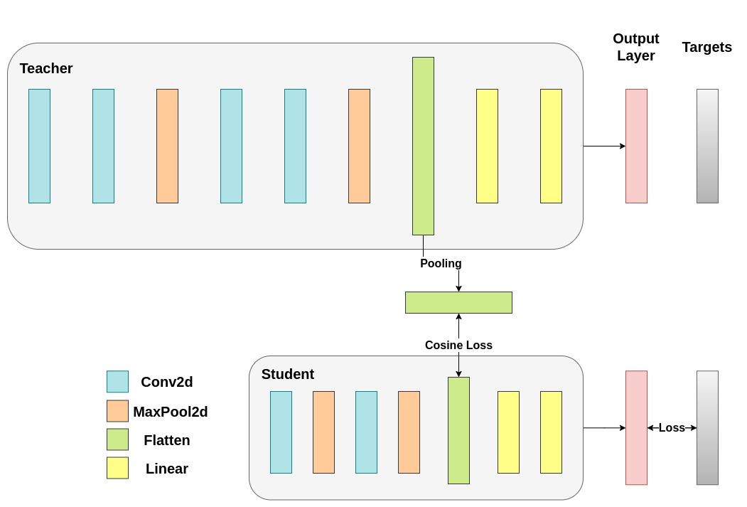
余弦损失最小化运行

请随意调整控制 softmax 函数柔和度的温度参数以及损失系数。在神经网络中，可以轻松地将额外的损失函数添加到主要目标中，以实现更好的泛化等目标。让我们尝试为学生的网络添加一个目标，但这次我们将关注它们的隐藏状态而非输出层。我们的目标是通过引入一个简单的损失函数，将教师网络的表示信息传递给学生网络，这个损失函数的最小化意味着随后传递给分类器的扁平化向量在损失减少时变得更加相似。当然，教师网络的权重不会更新，因此最小化仅依赖于学生网络的权重。这种方法背后的逻辑是，我们假设教师模型具有更好的内部表示，而学生网络在没有外部干预的情况下不太可能达到这种表示，因此我们人为地推动学生网络模仿教师网络的内部表示。然而，这是否最终会帮助学生网络并不明确，因为推动轻量级网络达到这一点可能是好事，假设我们找到了一个能带来更好测试精度的内部表示，但也可能是有害的，因为网络架构不同，学生网络的学习能力不如教师网络。换句话说，学生网络和教师网络的这两个向量没有理由在每个分量上都匹配。学生网络可能达到一个与教师网络内部表示排列不同的表示，但同样高效。尽管如此，我们仍然可以快速进行实验以了解这种方法的影响。我们将使用 CosineEmbeddingLoss，其公式如下：

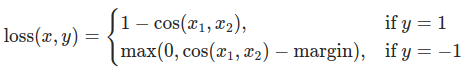
CosineEmbeddingLoss 的公式

显然，我们需要先解决一个问题。当我们对输出层应用蒸馏时，我们提到两个网络具有相同数量的神经元，即等于类别数。然而，对于卷积层之后的层来说，情况并非如此。在这里，教师在最后一个卷积层展平后比学生拥有更多的神经元。我们的损失函数接受两个维度相同的向量作为输入，因此我们需要以某种方式使它们匹配。我们将在教师的卷积层之后添加一个平均池化层，以降低其维度，使其与学生的维度相匹配。

接下来，我们将修改或创建新的模型类。现在，forward 函数不仅返回网络的 logits，还返回卷积层后的展平隐藏表示。我们在修改后的教师模型中包含了上述的池化操作。

classModifiedDeepNNCosine(nn.Module):
    def__init__(self, num_classes=10):
        super(ModifiedDeepNNCosine, self).__init__()
        self.features = nn.Sequential(
            nn.Conv2d(3, 128, kernel_size=3, padding=1),
            nn.ReLU(),
            nn.Conv2d(128, 64, kernel_size=3, padding=1),
            nn.ReLU(),
            nn.MaxPool2d(kernel_size=2, stride=2),
            nn.Conv2d(64, 64, kernel_size=3, padding=1),
            nn.ReLU(),
            nn.Conv2d(64, 32, kernel_size=3, padding=1),
            nn.ReLU(),
            nn.MaxPool2d(kernel_size=2, stride=2),
        )
        self.classifier = nn.Sequential(
            nn.Linear(2048, 512),
            nn.ReLU(),
            nn.Dropout(0.1),
            nn.Linear(512, num_classes)
        )

    defforward(self, x):
        x = self.features(x)
        flattened_conv_output = torch.flatten(x, 1)
        x = self.classifier(flattened_conv_output)
        flattened_conv_output_after_pooling = torch.nn.functional.avg_pool1d(flattened_conv_output, 2)
        return x, flattened_conv_output_after_pooling

# Create a similar student class where we return a tuple. We do not apply pooling after flattening.
classModifiedLightNNCosine(nn.Module):
    def__init__(self, num_classes=10):
        super(ModifiedLightNNCosine, self).__init__()
        self.features = nn.Sequential(
            nn.Conv2d(3, 16, kernel_size=3, padding=1),
            nn.ReLU(),
            nn.MaxPool2d(kernel_size=2, stride=2),
            nn.Conv2d(16, 16, kernel_size=3, padding=1),
            nn.ReLU(),
            nn.MaxPool2d(kernel_size=2, stride=2),
        )
        self.classifier = nn.Sequential(
            nn.Linear(1024, 256),
            nn.ReLU(),
            nn.Dropout(0.1),
            nn.Linear(256, num_classes)
        )

    defforward(self, x):
        x = self.features(x)
        flattened_conv_output = torch.flatten(x, 1)
        x = self.classifier(flattened_conv_output)
        return x, flattened_conv_output

# We do not have to train the modified deep network from scratch of course, we just load its weights from the trained instance
modified_nn_deep = ModifiedDeepNNCosine(num_classes=10).to(device)
modified_nn_deep.load_state_dict(nn_deep.state_dict())

# Once again ensure the norm of the first layer is the same for both networks
print("Norm of 1st layer for deep_nn:", torch.norm(nn_deep.features[0].weight).item())
print("Norm of 1st layer for modified_deep_nn:", torch.norm(modified_nn_deep.features[0].weight).item())

# Initialize a modified lightweight network with the same seed as our other lightweight instances. This will be trained from scratch to examine the effectiveness of cosine loss minimization.
torch.manual_seed(42)
modified_nn_light = ModifiedLightNNCosine(num_classes=10).to(device)
print("Norm of 1st layer:", torch.norm(modified_nn_light.features[0].weight).item())

Norm of 1st layer for deep_nn: 7.470613956451416
Norm of 1st layer for modified_deep_nn: 7.470613956451416
Norm of 1st layer: 2.327361822128296

自然地，我们需要修改训练循环，因为现在模型返回的是一个元组 (logits, hidden_representation)。通过使用一个示例输入张量，我们可以打印它们的形状。

# Create a sample input tensor
sample_input = torch.randn(128, 3, 32, 32).to(device) # Batch size: 128, Filters: 3, Image size: 32x32

# Pass the input through the student
logits, hidden_representation = modified_nn_light(sample_input)

# Print the shapes of the tensors
print("Student logits shape:", logits.shape) # batch_size x total_classes
print("Student hidden representation shape:", hidden_representation.shape) # batch_size x hidden_representation_size

# Pass the input through the teacher
logits, hidden_representation = modified_nn_deep(sample_input)

# Print the shapes of the tensors
print("Teacher logits shape:", logits.shape) # batch_size x total_classes
print("Teacher hidden representation shape:", hidden_representation.shape) # batch_size x hidden_representation_size

Student logits shape: torch.Size([128, 10])
Student hidden representation shape: torch.Size([128, 1024])
Teacher logits shape: torch.Size([128, 10])
Teacher hidden representation shape: torch.Size([128, 1024])

在我们的例子中，hidden_representation_size 为 1024。这是学生模型的最后一个卷积层的展平特征图，正如你所见，它也是学生分类器的输入。对于教师模型，它也是 1024，因为我们通过 avg_pool1d 从 2048 进行了调整。这里应用的损失仅在计算损失之前影响学生模型的权重。换句话说，它不会影响学生模型的分类器。修改后的训练循环如下：

../_static/img/knowledge_distillation/cosine_loss_distillation.png

在余弦损失最小化中，我们希望通过向学生模型返回梯度来最大化两种表示的余弦相似度：

deftrain_cosine_loss(teacher, student, train_loader, epochs, learning_rate, hidden_rep_loss_weight, ce_loss_weight, device):
    ce_loss = nn.CrossEntropyLoss()
    cosine_loss = nn.CosineEmbeddingLoss()
    optimizer = optim.Adam(student.parameters(), lr=learning_rate)

    teacher.to(device)
    student.to(device)
    teacher.eval()  # Teacher set to evaluation mode
    student.train() # Student to train mode

    for epoch in range(epochs):
        running_loss = 0.0
        for inputs, labels in train_loader:
            inputs, labels = inputs.to(device), labels.to(device)

            optimizer.zero_grad()

            # Forward pass with the teacher model and keep only the hidden representation
            with torch.no_grad():
                _, teacher_hidden_representation = teacher(inputs)

            # Forward pass with the student model
            student_logits, student_hidden_representation = student(inputs)

            # Calculate the cosine loss. Target is a vector of ones. From the loss formula above we can see that is the case where loss minimization leads to cosine similarity increase.
            hidden_rep_loss = cosine_loss(student_hidden_representation, teacher_hidden_representation, target=torch.ones(inputs.size(0)).to(device))

            # Calculate the true label loss
            label_loss = ce_loss(student_logits, labels)

            # Weighted sum of the two losses
            loss = hidden_rep_loss_weight * hidden_rep_loss + ce_loss_weight * label_loss

            loss.backward()
            optimizer.step()

            running_loss += loss.item()

        print(f"Epoch {epoch+1}/{epochs}, Loss: {running_loss/len(train_loader)}")

出于同样的原因，我们需要修改我们的测试函数。在这里，我们忽略了模型返回的隐藏表示。

deftest_multiple_outputs(model, test_loader, device):
    model.to(device)
    model.eval()

    correct = 0
    total = 0

    with torch.no_grad():
        for inputs, labels in test_loader:
            inputs, labels = inputs.to(device), labels.to(device)

            outputs, _ = model(inputs) # Disregard the second tensor of the tuple
            _, predicted = torch.max(outputs.data, 1)

            total += labels.size(0)
            correct += (predicted == labels).sum().item()

    accuracy = 100 * correct / total
    print(f"Test Accuracy: {accuracy:.2f}%")
    return accuracy

在这种情况下，我们可以轻松地在同一个函数中包含知识蒸馏和余弦损失最小化。通常，在教师-学生范式中，结合多种方法以实现更好的性能是很常见的。现在，我们可以运行一个简单的训练-测试会话。

# Train and test the lightweight network with cross entropy loss
train_cosine_loss(teacher=modified_nn_deep, student=modified_nn_light, train_loader=train_loader, epochs=10, learning_rate=0.001, hidden_rep_loss_weight=0.25, ce_loss_weight=0.75, device=device)
test_accuracy_light_ce_and_cosine_loss = test_multiple_outputs(modified_nn_light, test_loader, device)

Epoch 1/10, Loss: 1.3078211134352038
Epoch 2/10, Loss: 1.0733076152594194
Epoch 3/10, Loss: 0.9724330520995742
Epoch 4/10, Loss: 0.8980446970066451
Epoch 5/10, Loss: 0.844770607283658
Epoch 6/10, Loss: 0.7975365897578657
Epoch 7/10, Loss: 0.7560262779140716
Epoch 8/10, Loss: 0.7221040294298431
Epoch 9/10, Loss: 0.6851439026310621
Epoch 10/10, Loss: 0.6586272847621947
Test Accuracy: 70.48%

中间回归器运行

我们的简单最小化操作并不能保证更好的结果，原因有多方面，其中之一是向量的维度。对于高维向量，余弦相似度通常比欧几里得距离效果更好，但我们处理的是每个向量有 1024 个分量的情况，因此提取有意义的相似性要困难得多。此外，正如我们所提到的，推动教师模型和学生模型的隐藏表示匹配并没有理论支持。没有充分的理由说明我们应该追求这些向量的 1:1 匹配。我们将通过引入一个称为回归器的额外网络，提供一个训练干预的最终示例。其目标是首先提取教师模型在卷积层后的特征图，然后提取学生模型在卷积层后的特征图，最后尝试匹配这些特征图。然而，这一次我们将在网络之间引入一个回归器，以促进匹配过程。回归器是可训练的，理想情况下它将比我们简单的余弦损失最小化方案做得更好。它的主要工作是匹配这些特征图的维度，以便我们能够正确定义教师模型和学生模型之间的损失函数。定义这样的损失函数提供了一个“教学路径”，本质上是一个反向传播梯度的流程，它将改变学生模型的权重。关注我们原始网络中每个分类器之前的卷积层输出，我们得到以下形状：

# Pass the sample input only from the convolutional feature extractor
convolutional_fe_output_student = nn_light.features(sample_input)
convolutional_fe_output_teacher = nn_deep.features(sample_input)

# Print their shapes
print("Student's feature extractor output shape: ", convolutional_fe_output_student.shape)
print("Teacher's feature extractor output shape: ", convolutional_fe_output_teacher.shape)

Student's feature extractor output shape:  torch.Size([128, 16, 8, 8])
Teacher's feature extractor output shape:  torch.Size([128, 32, 8, 8])

我们为教师模型配置了32个过滤器，为学生模型配置了16个过滤器。我们将引入一个可训练的层，用于将学生模型的特征图转换为教师模型特征图的形状。在实际操作中，我们调整了轻量级类，使其在经过一个中间回归器后返回隐藏状态，该回归器用于匹配卷积特征图的大小，同时调整教师类，使其返回最终卷积层的输出，无需进行池化或展平处理。

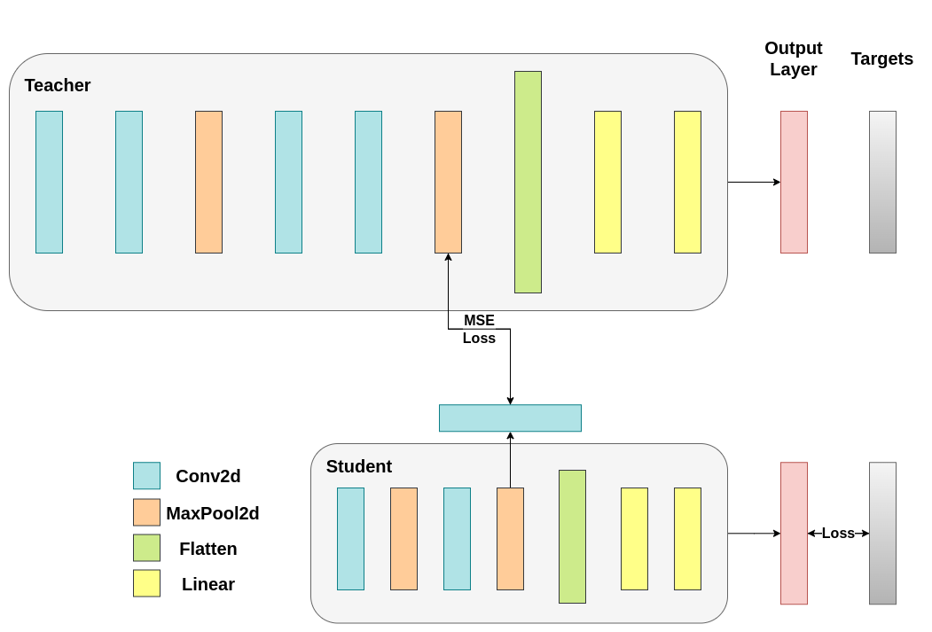
../_static/img/knowledge_distillation/fitnets_knowledge_distill.png

可训练层匹配中间张量的形状，并且均方误差（MSE）正确定义：

classModifiedDeepNNRegressor(nn.Module):
    def__init__(self, num_classes=10):
        super(ModifiedDeepNNRegressor, self).__init__()
        self.features = nn.Sequential(
            nn.Conv2d(3, 128, kernel_size=3, padding=1),
            nn.ReLU(),
            nn.Conv2d(128, 64, kernel_size=3, padding=1),
            nn.ReLU(),
            nn.MaxPool2d(kernel_size=2, stride=2),
            nn.Conv2d(64, 64, kernel_size=3, padding=1),
            nn.ReLU(),
            nn.Conv2d(64, 32, kernel_size=3, padding=1),
            nn.ReLU(),
            nn.MaxPool2d(kernel_size=2, stride=2),
        )
        self.classifier = nn.Sequential(
            nn.Linear(2048, 512),
            nn.ReLU(),
            nn.Dropout(0.1),
            nn.Linear(512, num_classes)
        )

    defforward(self, x):
        x = self.features(x)
        conv_feature_map = x
        x = torch.flatten(x, 1)
        x = self.classifier(x)
        return x, conv_feature_map

classModifiedLightNNRegressor(nn.Module):
    def__init__(self, num_classes=10):
        super(ModifiedLightNNRegressor, self).__init__()
        self.features = nn.Sequential(
            nn.Conv2d(3, 16, kernel_size=3, padding=1),
            nn.ReLU(),
            nn.MaxPool2d(kernel_size=2, stride=2),
            nn.Conv2d(16, 16, kernel_size=3, padding=1),
            nn.ReLU(),
            nn.MaxPool2d(kernel_size=2, stride=2),
        )
        # Include an extra regressor (in our case linear)
        self.regressor = nn.Sequential(
            nn.Conv2d(16, 32, kernel_size=3, padding=1)
        )
        self.classifier = nn.Sequential(
            nn.Linear(1024, 256),
            nn.ReLU(),
            nn.Dropout(0.1),
            nn.Linear(256, num_classes)
        )

    defforward(self, x):
        x = self.features(x)
        regressor_output = self.regressor(x)
        x = torch.flatten(x, 1)
        x = self.classifier(x)
        return x, regressor_output

之后，我们需要再次更新训练循环。这次，我们提取学生的回归器输出和教师的特征图，在这些张量上计算 MSE（它们的形状完全相同，因此定义合理），并根据该损失反向传播梯度，同时还包括分类任务中常规的交叉熵损失。

deftrain_mse_loss(teacher, student, train_loader, epochs, learning_rate, feature_map_weight, ce_loss_weight, device):
    ce_loss = nn.CrossEntropyLoss()
    mse_loss = nn.MSELoss()
    optimizer = optim.Adam(student.parameters(), lr=learning_rate)

    teacher.to(device)
    student.to(device)
    teacher.eval()  # Teacher set to evaluation mode
    student.train() # Student to train mode

    for epoch in range(epochs):
        running_loss = 0.0
        for inputs, labels in train_loader:
            inputs, labels = inputs.to(device), labels.to(device)

            optimizer.zero_grad()

            # Again ignore teacher logits
            with torch.no_grad():
                _, teacher_feature_map = teacher(inputs)

            # Forward pass with the student model
            student_logits, regressor_feature_map = student(inputs)

            # Calculate the loss
            hidden_rep_loss = mse_loss(regressor_feature_map, teacher_feature_map)

            # Calculate the true label loss
            label_loss = ce_loss(student_logits, labels)

            # Weighted sum of the two losses
            loss = feature_map_weight * hidden_rep_loss + ce_loss_weight * label_loss

            loss.backward()
            optimizer.step()

            running_loss += loss.item()

        print(f"Epoch {epoch+1}/{epochs}, Loss: {running_loss/len(train_loader)}")

# Notice how our test function remains the same here with the one we used in our previous case. We only care about the actual outputs because we measure accuracy.

# Initialize a ModifiedLightNNRegressor
torch.manual_seed(42)
modified_nn_light_reg = ModifiedLightNNRegressor(num_classes=10).to(device)

# We do not have to train the modified deep network from scratch of course, we just load its weights from the trained instance
modified_nn_deep_reg = ModifiedDeepNNRegressor(num_classes=10).to(device)
modified_nn_deep_reg.load_state_dict(nn_deep.state_dict())

# Train and test once again
train_mse_loss(teacher=modified_nn_deep_reg, student=modified_nn_light_reg, train_loader=train_loader, epochs=10, learning_rate=0.001, feature_map_weight=0.25, ce_loss_weight=0.75, device=device)
test_accuracy_light_ce_and_mse_loss = test_multiple_outputs(modified_nn_light_reg, test_loader, device)

Epoch 1/10, Loss: 1.710898199654601
Epoch 2/10, Loss: 1.3363171050615628
Epoch 3/10, Loss: 1.192594036879137
Epoch 4/10, Loss: 1.1002179387280397
Epoch 5/10, Loss: 1.0243484219321815
Epoch 6/10, Loss: 0.963491040270042
Epoch 7/10, Loss: 0.9118528664874299
Epoch 8/10, Loss: 0.8608026291098436
Epoch 9/10, Loss: 0.8202611104301785
Epoch 10/10, Loss: 0.77916762286135
Test Accuracy: 70.43%

预期最终的方法会比 CosineLoss 表现得更好，因为现在我们在教师模型和学生模型之间加入了一个可训练的层，这为学生的学习提供了一定的灵活性，而不是强迫学生直接复制教师模型的表示。加入额外的网络是基于提示的蒸馏（hint-based distillation）背后的核心思想。

print(f"Teacher accuracy: {test_accuracy_deep:.2f}%")
print(f"Student accuracy without teacher: {test_accuracy_light_ce:.2f}%")
print(f"Student accuracy with CE + KD: {test_accuracy_light_ce_and_kd:.2f}%")
print(f"Student accuracy with CE + CosineLoss: {test_accuracy_light_ce_and_cosine_loss:.2f}%")
print(f"Student accuracy with CE + RegressorMSE: {test_accuracy_light_ce_and_mse_loss:.2f}%")

Teacher accuracy: 74.59%
Student accuracy without teacher: 70.66%
Student accuracy with CE + KD: 70.63%
Student accuracy with CE + CosineLoss: 70.48%
Student accuracy with CE + RegressorMSE: 70.43%

结论

上述方法均未增加网络的参数数量或推理时间，因此性能的提升仅需在训练时计算梯度的微小代价。在机器学习应用中，我们主要关注推理时间，因为训练发生在模型部署之前。如果我们的轻量级模型在部署时仍然过于庞大，我们可以采用不同的思路，例如训练后量化。额外的损失可以应用于许多任务，而不仅仅是分类，并且你可以尝试调整系数、温度或神经元数量等参数。请随意调整上述教程中的任何数值，但请注意，如果更改神经元/过滤器的数量，可能会导致形状不匹配的情况发生。

下载 Jupyter 笔记本: knowledge_distillation_tutorial.ipynb