NLP从零开始:用字符级RNN进行姓名分类
作者: Sean Robertson
我们将构建并训练一个基本的字符级循环神经网络(RNN)来分类单词。本教程与另外两个从零开始的自然语言处理(NLP)教程 从零开始的 NLP:使用字符级 RNN 生成名称 和 从零开始的 NLP:使用序列到序列网络和注意力机制进行翻译,展示了如何预处理数据以用于 NLP 建模。特别是这些教程没有使用torchtext 的许多便捷函数,因此你可以看到在低级别下预处理 NLP 数据的方法。
字符级的循环神经网络(RNN)将单词视为一系列字符进行处理,在每个时间步输出预测结果和“隐藏状态”,并将其前一个隐藏状态传递给下一个时间步。我们取最终的预测结果作为输出,即该单词所属的类别。
具体来说,我们将使用来自18个不同来源语言的几千个姓氏进行训练,并根据拼写预测姓名所属的语言。
$pythonpredict.pyHinton
(-0.47)Scottish
(-1.52)English
(-3.57)Irish

$pythonpredict.pySchmidhuber
(-0.19)German
(-2.48)Czech
(-2.68)Dutch
推荐准备工作
-
https://pytorch.org/ 提供了安装说明
-
使用PyTorch进行深度学习:60分钟速成,以快速入门PyTorch并学习张量的基础知识。
-
使用示例学习 PyTorch,以获得全面而深入的了解
-
PyTorch 实用技巧:Former Torch 用户指南(如果你是 Former Lua Torch 用户)
了解循环神经网络(RNN)及其工作原理也会很有用:
-
循环神经网络的不合理有效性展示了大量的现实生活中的实例。
-
理解LSTM网络专门介绍LSTMs,但同时也为一般RNNs提供了有价值的参考信息。
准备数据
注
从这里下载数据,并将其解压到当前目录。
在 data/names 目录中包含了 18 个名为 [Language].txt 的文本文件。每个文件包含了一系列的名字,每行一个名字,大多数是罗马化形式(但我们需要将它们从 Unicode 转换为 ASCII)。
我们将得到一个按语言分类的名字列表字典,{language: [names ...]}。这里的通用变量“category”和“line”(在我们的例子中分别表示“语言”和“名字”)用于后续的扩展。
from io import open
import glob
import os

def findFiles(path): return glob.glob(path)

print(findFiles('data/names/*.txt'))

import unicodedata
import string

all_letters = string.ascii_letters + " .,;'"
n_letters = len(all_letters)

# Turn a Unicode string to plain ASCII, thanks to https://stackoverflow.com/a/518232/2809427
def unicodeToAscii(s):
    return ''.join(
        c for c in unicodedata.normalize('NFD', s)
        if unicodedata.category(c) != 'Mn'
        and c in all_letters
    )

print(unicodeToAscii('Ślusàrski'))

# Build the category_lines dictionary, a list of names per language
category_lines = {}
all_categories = []

# Read a file and split into lines
def readLines(filename):
    lines = open(filename, encoding='utf-8').read().strip().split('\n')
    return [unicodeToAscii(line) for line in lines]

for filename in findFiles('data/names/*.txt'):
    category = os.path.splitext(os.path.basename(filename))[0]
    all_categories.append(category)
    lines = readLines(filename)
    category_lines[category] = lines

n_categories = len(all_categories)
['data/names/Arabic.txt', 'data/names/Chinese.txt', 'data/names/Czech.txt', 'data/names/Dutch.txt', 'data/names/English.txt', 'data/names/French.txt', 'data/names/German.txt', 'data/names/Greek.txt', 'data/names/Irish.txt', 'data/names/Italian.txt', 'data/names/Japanese.txt', 'data/names/Korean.txt', 'data/names/Polish.txt', 'data/names/Portuguese.txt', 'data/names/Russian.txt', 'data/names/Scottish.txt', 'data/names/Spanish.txt', 'data/names/Vietnamese.txt']
Slusarski
现在我们有了一个将每个类别(语言)映射到行列表(名称)的字典 category_lines。我们也记录了变量 all_categories(即语言列表)和 n_categories,以备后用。
print(category_lines['Italian'][:5])
['Abandonato', 'Abatangelo', 'Abatantuono', 'Abate', 'Abategiovanni']
将名称转化为张量
为了表示单个字母,我们使用大小为 <1 x n_letters> 的“one-hot 向量”。一个 one-hot 向量除了当前字母的索引位置是 1 外,其余位置都是 0,例如 "b" = <0 1 0 0 0 ...>。
要构成一个词,我们将这些元素组合成一个二维矩阵<line_length x 1 x n_letters>。
那个额外的维度是因为 PyTorch 假设所有数据都是以批的形式处理的,而这里我们只是使用了一个大小为 1 的批次。
import torch

# Find letter index from all_letters, e.g. "a" = 0
def letterToIndex(letter):
    return all_letters.find(letter)

# Just for demonstration, turn a letter into a <1 x n_letters> Tensor
def letterToTensor(letter):
    tensor = torch.zeros(1, n_letters)
    tensor[0][letterToIndex(letter)] = 1
    return tensor

# Turn a line into a <line_length x 1 x n_letters>,
# or an array of one-hot letter vectors
def lineToTensor(line):
    tensor = torch.zeros(len(line), 1, n_letters)
    for li, letter in enumerate(line):
        tensor[li][0][letterToIndex(letter)] = 1
    return tensor

print(letterToTensor('J'))

print(lineToTensor('Jones').size())
tensor([[0., 0., 0., 0., 0., 0., 0., 0., 0., 0., 0., 0., 0., 0., 0., 0., 0., 0.,
         0., 0., 0., 0., 0., 0., 0., 0., 0., 0., 0., 0., 0., 0., 0., 0., 0., 1.,
         0., 0., 0., 0., 0., 0., 0., 0., 0., 0., 0., 0., 0., 0., 0., 0., 0., 0.,
         0., 0., 0.]])
torch.Size([5, 1, 57])
创建网络
在自动微分功能实现之前,在Torch中创建循环神经网络需要在多个时间步长内克隆层的参数。这些层原本负责维护隐藏状态和梯度信息,而现在这些都完全由计算图本身来处理了。这意味着你可以用一种非常“纯粹”的方式来实现RNN,就像普通的前馈层一样。
这个 RNN 模块实现了一个“常规 RNN”,包含三个线性层,它们对输入和隐藏状态进行操作,并在输出后添加一个 LogSoftmax 层。
import torch.nn as nn
import torch.nn.functional as F

class RNN(nn.Module):
    def __init__(self, input_size, hidden_size, output_size):
        super(RNN, self).__init__()

        self.hidden_size = hidden_size

        self.i2h = nn.Linear(input_size, hidden_size)
        self.h2h = nn.Linear(hidden_size, hidden_size)
        self.h2o = nn.Linear(hidden_size, output_size)
        self.softmax = nn.LogSoftmax(dim=1)

    def forward(self, input, hidden):
        hidden = F.tanh(self.i2h(input) + self.h2h(hidden))
        output = self.h2o(hidden)
        output = self.softmax(output)
        return output, hidden

    def initHidden(self):
        return torch.zeros(1, self.hidden_size)

n_hidden = 128
rnn = RNN(n_letters, n_hidden, n_categories)
要运行此网络的一个步骤,我们需要传递一个输入(在这种情况下是当前字母的张量)以及初始值为零的先前隐藏状态。我们将会获得输出(即每种语言的概率),并保存下一个隐藏状态以供后续步骤使用。
input = letterToTensor('A')
hidden = torch.zeros(1, n_hidden)

output, next_hidden = rnn(input, hidden)
lineToTensor 替代 letterToTensor,并通过切片来实现。此外,还可以通过预计算张量批次进一步优化。
input = lineToTensor('Albert')
hidden = torch.zeros(1, n_hidden)

output, next_hidden = rnn(input[0], hidden)
print(output)
tensor([[-3.0014, -2.8677, -2.9758, -2.9196, -3.1387, -2.8728, -2.8886, -2.8754,
         -2.5694, -2.8957, -2.8363, -2.9602, -2.9206, -2.8656, -2.8350, -2.7372,
         -3.0470, -2.9479]], grad_fn=<LogSoftmaxBackward0>)
如你所见,输出是一个<1 x n_categories>的张量,每个元素表示相应类别被预测的概率,数值越大表示可能性越高。
培训
训练前的准备
Tensor.topk来获取最大值的索引。
('Irish', 8)
我们也希望能快速获取一个训练样本(包括名称和其对应的语言)。
import random

def randomChoice(l):
    return l[random.randint(0, len(l) - 1)]

def randomTrainingExample():
    category = randomChoice(all_categories)
    line = randomChoice(category_lines[category])
    category_tensor = torch.tensor([all_categories.index(category)], dtype=torch.long)
    line_tensor = lineToTensor(line)
    return category, line, category_tensor, line_tensor

for i in range(10):
    category, line, category_tensor, line_tensor = randomTrainingExample()
    print('category =', category, '/ line =', line)
category = Chinese / line = Hou
category = Scottish / line = Mckay
category = Arabic / line = Cham
category = Russian / line = V'Yurkov
category = Irish / line = O'Keeffe
category = French / line = Belrose
category = Spanish / line = Silva
category = Japanese / line = Fuchida
category = Greek / line = Tsahalis
category = Korean / line = Chang
训练网络
现在要训练这个网络,只需要向它展示一组示例,让它进行猜测,并告知它哪里出错即可。
由于RNN的最后一个层是nn.LogSoftmax,因此对于损失函数来说,使用nn.NLLLoss是合适的。
criterion = nn.NLLLoss()
每个训练循环将会:
-
创建输入和目标张量
-
创建一个初始隐藏状态为零的隐态
-
读取每个字母
-
保存下一个字母的隐藏状态
-
-
将最终输出与目标进行对比
-
反向传播
-
返回输出和损失值
learning_rate = 0.005 # If you set this too high, it might explode. If too low, it might not learn

def train(category_tensor, line_tensor):
    hidden = rnn.initHidden()

    rnn.zero_grad()

    for i in range(line_tensor.size()[0]):
        output, hidden = rnn(line_tensor[i], hidden)

    loss = criterion(output, category_tensor)
    loss.backward()

    # Add parameters' gradients to their values, multiplied by learning rate
    for p in rnn.parameters():
        p.data.add_(p.grad.data, alpha=-learning_rate)

    return output, loss.item()
现在我们只需要用大量的示例来运行它。由于 train 函数返回输出和损失,我们可以打印其猜测结果,并跟踪损失以供绘图。由于有成千上万个示例,我们只在每print_every个示例时进行一次打印,并取损失的平均值。
import time
import math

n_iters = 100000
print_every = 5000
plot_every = 1000


# Keep track of losses for plotting
current_loss = 0
all_losses = []

def timeSince(since):
    now = time.time()
    s = now - since
    m = math.floor(s / 60)
    s -= m * 60
    return '%dm %ds' % (m, s)

start = time.time()

for iter in range(1, n_iters + 1):
    category, line, category_tensor, line_tensor = randomTrainingExample()
    output, loss = train(category_tensor, line_tensor)
    current_loss += loss

    # Print ``iter`` number, loss, name and guess
    if iter % print_every == 0:
        guess, guess_i = categoryFromOutput(output)
        correct = '✓' if guess == category else '✗ (%s)' % category
        print('%d%d%% (%s) %.4f%s / %s%s' % (iter, iter / n_iters * 100, timeSince(start), loss, line, guess, correct))

    # Add current loss avg to list of losses
    if iter % plot_every == 0:
        all_losses.append(current_loss / plot_every)
        current_loss = 0
5000 5% (0m 17s) 2.2208 Horigome / Japanese ✓
10000 10% (0m 35s) 1.6752 Miazga / Japanese ✗ (Polish)
15000 15% (0m 53s) 0.1778 Yukhvidov / Russian ✓
20000 20% (1m 11s) 1.5856 Mclaughlin / Irish ✗ (Scottish)
25000 25% (1m 29s) 0.6552 Banh / Vietnamese ✓
30000 30% (1m 47s) 1.5547 Machado / Japanese ✗ (Portuguese)
35000 35% (2m 5s) 0.0168 Fotopoulos / Greek ✓
40000 40% (2m 23s) 1.1464 Quirke / Irish ✓
45000 45% (2m 41s) 1.7532 Reier / French ✗ (German)
50000 50% (3m 0s) 0.8413 Hou / Chinese ✓
55000 55% (3m 18s) 0.8587 Duan / Vietnamese ✗ (Chinese)
60000 60% (3m 36s) 0.2047 Giang / Vietnamese ✓
65000 65% (3m 54s) 2.5534 Cober / French ✗ (Czech)
70000 70% (4m 12s) 1.5163 Mateus / Arabic ✗ (Portuguese)
75000 75% (4m 31s) 0.2217 Hamilton / Scottish ✓
80000 80% (4m 49s) 0.4456 Maessen / Dutch ✓
85000 85% (5m 7s) 0.0239 Gan / Chinese ✓
90000 90% (5m 25s) 0.0521 Bellomi / Italian ✓
95000 95% (5m 43s) 0.0867 Vozgov / Russian ✓
100000 100% (6m 1s) 0.2730 Tong / Vietnamese ✓
绘制结果
通过绘制 all_losses 中的历史损失情况,可以展示网络的学习过程:
import matplotlib.pyplot as plt
import matplotlib.ticker as ticker

plt.figure()
plt.plot(all_losses)
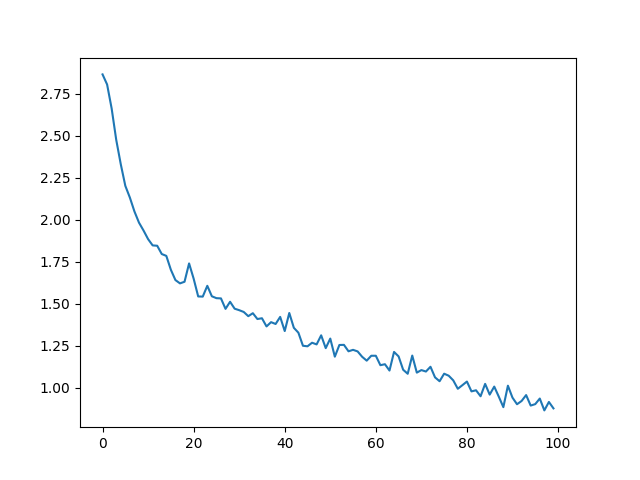
[<matplotlib.lines.Line2D object at 0x7f9dd159d5d0>]
评估结果
为了查看网络在不同类别上的表现,我们将创建一个混淆矩阵,表示对于每个实际语言(行),网络猜测的是哪种语言(列)。计算混淆矩阵时,需要将一批样本通过 evaluate() 函数运行,这与 train() 函数除去反向传播部分相同。
# Keep track of correct guesses in a confusion matrix
confusion = torch.zeros(n_categories, n_categories)
n_confusion = 10000

# Just return an output given a line
def evaluate(line_tensor):
    hidden = rnn.initHidden()

    for i in range(line_tensor.size()[0]):
        output, hidden = rnn(line_tensor[i], hidden)

    return output

# Go through a bunch of examples and record which are correctly guessed
for i in range(n_confusion):
    category, line, category_tensor, line_tensor = randomTrainingExample()
    output = evaluate(line_tensor)
    guess, guess_i = categoryFromOutput(output)
    category_i = all_categories.index(category)
    confusion[category_i][guess_i] += 1

# Normalize by dividing every row by its sum
for i in range(n_categories):
    confusion[i] = confusion[i] / confusion[i].sum()

# Set up plot
fig = plt.figure()
ax = fig.add_subplot(111)
cax = ax.matshow(confusion.numpy())
fig.colorbar(cax)

# Set up axes
ax.set_xticklabels([''] + all_categories, rotation=90)
ax.set_yticklabels([''] + all_categories)

# Force label at every tick
ax.xaxis.set_major_locator(ticker.MultipleLocator(1))
ax.yaxis.set_major_locator(ticker.MultipleLocator(1))

# sphinx_gallery_thumbnail_number = 2
plt.show()
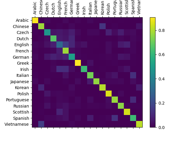
你可以挑选出主轴之外的亮点,显示它错误猜测的语言,例如将韩语误判为中文或将意大利语误判为西班牙语。它在识别希腊语方面表现出色,在识别英语方面则表现较差(可能是因为与其他语言有重叠)。
基于用户输入运行
def predict(input_line, n_predictions=3):
    print('\n> %s' % input_line)
    with torch.no_grad():
        output = evaluate(lineToTensor(input_line))

        # Get top N categories
        topv, topi = output.topk(n_predictions, 1, True)
        predictions = []

        for i in range(n_predictions):
            value = topv[0][i].item()
            category_index = topi[0][i].item()
            print('(%.2f) %s' % (value, all_categories[category_index]))
            predictions.append([value, all_categories[category_index]])

predict('Dovesky')
predict('Jackson')
predict('Satoshi')
> Dovesky
(-0.23) Czech
(-2.02) Russian
(-3.35) English

> Jackson
(-0.20) Scottish
(-2.51) Russian
(-3.05) Greek

> Satoshi
(-0.91) Italian
(-1.26) Japanese
(-1.57) Polish
Practical PyTorch 代码库中的最终版本的脚本将上述代码拆分到几个文件中:
-
data.py(负责加载文件) -
model.py(定义了RNN模型) -
train.py(用于运行训练) -
predict.py(通过命令行参数调用predict()) -
server.py(使用bottle.py将预测结果以 JSON API 的形式提供服务)
运行 train.py 来训练和保存网络。
通过运行 predict.py 并指定名称来查看预测结果。
$pythonpredict.pyHazaki
(-0.42)Japanese
(-1.39)Polish
(-3.51)Czech
运行 server.py,然后访问 http://localhost:5533/Yourname 查看预测结果的 JSON 输出。
练习
-
尝试使用不同的数据集,例如:线→类别:
-
任何词 -> 语言
-
姓名 -> 性别
-
角色名称 -> 作者
-
页面标题 -> 博客或 subreddit
-
-
通过使用更大或更优结构的网络,获得更好的结果
-
添加更多的线性层
-
尝试使用
nn.LSTM和nn.GRU层 -
将多个这样的RNN结合起来形成一个更高层次的网络
-